by Robert P. Murphy

[Reprinted from the December 2018 edition of the Lara-Murphy-Report, LMR]

One Of the most common questions we get from the public is whether IBC “works” or “makes sense” for someone who is older and/or in relatively poor health. People naturally worry whether the “pure cost of life insurance”—which is more expensive for older and/or sicker individuals, of course— at some point could make IBC impractical. If so, would it be better for people in this situation to take out IBC policies on others who are younger and/or in better health?

My short answer is: no. Generally speaking, IBC “works” for anybody. To a first approximation, the higher mortality rate of an insured party has two opposing forces that roughly cancel out, as far as IBC goes: On the one hand, to achieve a desired death benefit level, an older and/or sicker person will have to pay a higher premium. But on the other hand, since that person is more likely to die, the cash value of that policy at any moment will be higher, than an otherwise comparable policy for a younger and/or healthier person. (Think of it this way: the life insurance company would be willing to pay an older/sicker person more to surrender a policy of a certain death benefit, than it would pay to a younger/healthier person to surrender a policy of the same death benefit.)

Now it’s true that the growth rate of the cash value will—other things equal—be lower for the older/sicker person, but that is counterbalanced by the fact that there’s always a greater chance of such a person dying and achieving the death benefit earlier. Once you take into account all of the relevant variables, the true “financial value” of funding a whole life policy on different types of people isn’t directly dependent on the age or health status of the individuals being insured.

To sum up, in terms of the big picture, yes, a person who’s older/sicker will have to pay higher premiums for a certain amount of death benefit coverage. But those higher premiums will be associated with larger cash values too. The cash value will tend to grow faster for the younger/healthier person (other things equal), but the market value of having such a policy in force is correspondingly lower, since there is less chance of getting the death benefit. To the extent that one also wants to use a life insurance policy as a cashflow management system—i.e. if you want to “become your own banker” as Nelson Nash recommends—then the various forces largely cancel out. You can effectively implement IBC with a dividend-paying whole life insurance policy, regardless of the age or health status of the person being insured (assuming the person can obtain a policy in the first place).

A Numerical Example

We have many experts in IBC who subscribe to the Lara-Murphy Report, including financial professionals and even insurance actuaries. So, with apologies to the casual reader who just wants bottomline “news you can use,” let me take the time to walk through a particular numerical example, illustrating the general principles I stated above.

Now the calculations in these types of analyses can get really complicated, really quickly. So in this article I’m going to make it as simple as possible, while still retaining the essence of our topic. To that end, I’m going to sweep away all of the overhead expenses—things like paying the salaries of the secretaries and maintenance staff for the home office—and simply assume that the life insurance company charges the actuarially fair premiums on the policies we will analyze. This is obviously unrealistic, but it makes our analysis very pure and crisp, so that we can isolate how an individual’s mortality rate affects the desirability of IBC.

Specifically, we’re going to look at a single-pay whole life insurance policy with a $1 million death benefit. The first applicant is Healthy Hank, while the second applicant is Sickly Sam. They are both 116 years old when they apply for their respective policies. The contract specifies that each applicant will make a one-time premium payment at the start of the policy, after which the policy is fully funded. (Note that in this article, I’m not worrying about turning the policy into a Modified Endowment Contract [MEC] or other subtleties of real-world policy design. We’re just trying to keep the math as easy as possible to study the issue in question.)

Now each of these policies is designed to “mature” at age 121. In other words, even if the applicant is still alive, if he reaches age 121 then he gets paid the $1 million benefit. This reflects real-world contract design, and also gives our math problem a nice terminal point, so we don’t have to keep carrying out probabilities forever when computing the financial value of an in-force policy.

To keep things simple, we are also going to assume a constant annual discount rate of 5 percent. (Think of this as the going rate of return on very safe bonds.) In these types of calculations, we need to take into consideration the time value of money, and for our purposes we’ll just assume a 5 percent annual interest rate.

With that framework in mind, Table 1 presents the theoretical cash surrender values for the policies on Sickly Sam and Healthy Hank, as well as the market values of a safe, zero-coupon bond that has a face maturity value of $1 million.

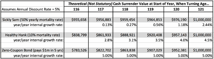
Table 1. Theoretical Values for Two Whole Life Policies and a Safe Bond

The calculations underlying Table 1 are quite elementary, meaning that the interested reader can recreate it in Excel and explore other scenarios. Here, I’ll explain just a few of the numbers to illustrate the pattern.

It’s easiest to start at the end. Clearly, the market values of all three of our financial instruments will be precisely $1 million at the start of the year when Sam and Hank turn 121. Their respective whole life policies “mature” or “endow” at that point, even if they are still breathing, and so they receive the contractual $1 million in “death benefit.” Like-wise, the holder of the bond at that moment also receives a cash payout of $1 million, and so the market value of the bond (seconds before payment) must also be $1 million.

Now let’s go back one year, to when the men just turn 120 years old. The bond’s present-discounted market value is simply $1 million divided by 1.05, which works out to $952,381 (rounding to the nearest dollar). Going the other way, if you start with $952,381 in Year 120 and invest it to earn 5% in the bond market, you will end up with $952,381 x 1.05 =~ $1 million in Year 121.

But now we move on to the more difficult computations. What is the theoretical cash surrender value for Sickly Sam’s whole life policy, at the start of Year 120? (And by theoretical, I mean: according to textbook theory, just worrying about the pure, actuarially fair cost of life insurance, and the going market rate of interest. We’re not worried about real-world statutory regulations or overhead expenses, agent commissions, etc.)

The textbook definition of the cash surrender value is something like: the present-discounted value of the actuarially expected death benefit, minus the present value of the expected flow of future premium payments. As time passes, the cash value on a policy rises, because: (a) the looming death benefit gets closer and closer, rising in present-value terms, and (b) with each premium payment made, there is one fewer such payment due in the future acting as a “lien” against the death benefit.

In Table 1, though, I have made the cash value as simple as possible to compute, because we assume the only premium payment is made once, on the front end. So at any given time, the theoretical cash surrender value is simply the $1 million death benefit, adjusted for the likelihood of payout (because of mortality) and the time value of money.

Calculating Specific Cash Surrender Values in Earlier Years

Let’s return now to Year 120, and actually calculate the cash surrender values for our two policies. First, start with Sickly Sam. At the beginning of Year 120, there is a metaphorical coin toss, with a 50-50 chance that Sam dies and gets the full $1 million death benefit right away. Or, there’s a 50-50 chance that Sam survives the year, reaching age 121 and then (at that time, twelve months in the future) gets the $1 million payout.

(For purists, note that I am making this calculation easier than it would be in real life. In reality, it’s not that individuals have a one-shot lottery at the start of each year, and they either die at that exact moment or live for another twelve months. But I want there to be only two components to each year’s calculation, so I’m assuming this unrealistic model for life/death.)

Returning to Sam, at the start of Year 120: We have calculated that there is a 50% chance his whole life policy pays $1 million right now, and a 50% chance that it will pay nothing now, and end up being worth $1 million in one year’s time. To compute the present-discounted market value of this asset, therefore, we say:

50% x $1 million + 50% x ($1 million)/1.05 =~ $976,190

Note that we had to discount the second term in the calculation by the prevailing discount rate of 5%, because that future cash surrender value is only available after waiting an additional year.

We’ll do one more calculation for Sam, to make sure you the reader understand how it works. If we go back yet another year, to the start of Age 119, we reckon that there is a 50% chance of getting the death benefit of $1 million right away (because Sam dies that year), plus a 50% chance that Sam lives un- til age 120, at which time the policy will be worth $976,190. We therefore compute:

50% x $1 million + 50% x ($976,190)/1.05 =~ $964,853 2

And so on, for the earlier values of Sickly Sam’s whole life policy.

Turning to Healthy Hank, we’ll calculate just the first number, to show the pattern. At the start of Year 120, there is a 10% chance that Hank will die, getting the immediate payout of $1 million. There is a 90% chance that Hank will survive the year, in order to get his hands on a policy with a $1 million cash surrender value twelve months later. Thus, the market value of his policy at the start of Year 120 is:

10% x $1 million + 90% x ($1 million)/1.05 =~ $957,143

And at this point, I trust that the reader can figure out how the other values in Table 1 are calculated.

Reflections on Table 1

Now that we’ve explained how Table 1 was built, let’s step back and consider its implications. In particular, does IBC “work better” for Healthy Hank than it does for Sickly Sam?

Obviously, Sam has to pay a higher one-shot premium. After all, he is much more likely to die in any given year than Healthy Hank, and—by construction—we designed policies that both have the same $1 million in death benefit coverage. So clearly, Sickly Sam’s premium payment will be higher. (Next month, in Part 2 of this series, I’ll consider a scenario where Sam and Hank make the same flow of premium payments, where their different mortality rates will then show up in different amounts of death benefit coverage.)

In our hypothetical example with no overhead expenses, to get into his policy, Sam would need to pay the “fair” market value of $955,658 at the start of Year 116, for a fully-paid up policy with a face death benefit of $1 million. In contrast, Healthy Hank only has to pay $838,799 for the same policy.

But notice that the available cash values—which they can obtain by surrendering the policy, or which can serve as collateral for policy loans—are different. Again, in our hypothetical world of no overhead or other frictions, the full single-pay premium is immediately reflected in the cash surrender value. So yes, Sickly Sam has to pay more for “the same” policy, but he has a higher cash surrender value right away. And notice this holds for the entire life of the policy, too: In every year during the development of the policies, Sam’s has a higher cash value than Hank’s. The men only have the same cash value at the very end, when both policies mature and reach $1 million in cash value.

In Part 2 of this series, I will go through a more complicated example, where Sickly Sam and Healthy Hank pay annual premiums on their whole life policies. But for our purposes in this introductory piece, I wanted there to be as few moving parts as possible. As Table 1 shows, Sickly Sam isn’t a fool for taking out an IBC policy on himself; all of his money goes toward his cash value, just as the case for Healthy Hank. It’s not the case that of his initial premium payment, Sam would see more of it “burned up by the pure cost of insurance,” compared to Hank, if what we mean by that is: How much of the initial premium payment showed up as cash value?

Let me shout once again from the rooftops: These are very simplistic calculations, relying only on hypothetical mortality rates and the market rate of interest. In the real world, there are many other factors at play. But in this article, I want to show the reader that your intuition about how “the pure cost of life insurance” interacts with premium payments and cash value, might not be correct.

“But What About the Internal Growth Rate? Isn’t Dave Ramsey Right After All?!”

At the risk of having some casual readers merely look at Table 1 without reading the article, I decided to include the annual growth rates of the market values of the three assets as well. A quick glance probably confirms the intuition of people who think, “Surely it’s less efficient to implement IBC on someone who’s older or in poor health, because there’s more ‘drag’ on the policy being eaten up by the higher pure cost of life insurance.”

And indeed, that does seem to jump out of Table 1, doesn’t it? After all, we can see that the growth rates of the cash surrender value for Sickly Sam are very modest, while they are much higher for Healthy Hank.3

And should Dave Ramsey happen to see this article, he would no doubt look at the even higher rates on the simple bond, and exclaim,“I told you so! You don’t want to use life insurance as an investment vehicle. The performance on the insurance company’s portfolio gets diluted by the pure cost of life insurance, and that’s especially true if you are older or sick.”

Not so fast. As I pointed out in my full response to his arguments about permanent life insurance—available in the September 2012 issue of the Lara-Murphy Report— Dave Ramsey disregards the financial value of having an in-force life insurance policy. Yes, looking at Table 1 and if we only worried about rates of return, you would be a fool to buy a whole life policy (rather than a bond) if you knew for sure that the insured party would live to age 121. But of course, a major element in a life insurance policy is that the insured party might die, entitling the beneficiary to the full death benefit ahead of Age 121.

To illustrate what I mean, let’s do a really simple comparison. Suppose Sickly Sam is in Year 120, and he’s trying to decide whether to put his money in a whole life policy on himself, or in a safe bond yielding 5 percent. A very naïve reader of Table 1 might advise Sam, “Clearly you should opt for the bond. Either way, you end up with $1 million, but the bond only costs you $952,381 to ‘get in’ at Year 120. Then you earn a 5% return, with the bond paying back $1 million a year later. In contrast, you have to pay a one-shot premium of $976,190 to get your whole life policy at age 120, in order for you to earn a mere 2.44% of internal growth before it matures and pays $1 million a year later. This is a no brainer.”

However, such advice is totally wrong. It overlooks the possibility that Sickly Sam dies in Year 120. In that event, the bond doesn’t do anything special; it still pays $1 million the next year. But the life insurance policy pays $1 million right away, and the person running Sam’s estate can then invest it for the prevailing 5% return in the market, yielding $1,050,000 the next year.

Thus, at the start of Year 120, if Sam buys the whole life policy, he expects: (A) a 50% chance of dying and ending up with $1,050,000 in his estate a year later, and (B) a 50% chance of living and getting $1 million a year later. The statistically “expected” value of this investment would therefore be $1,025,000, in the Year 121.

And now the grand finale: Sam, at the start of Year 120, has just calculated that in one year’s time, his life insurance policy will cause his estate to have a statistically expected $1,025,000 extra. And what is the present value of that future possibility? Well he just discounts it by the interest rate, to calculate $1,025,000 / 1.05 =~ $976,190, which is exactly what Table 1 shows is the actuarially fair cash surrender value / single-pay premium payment for this policy.

IBC isn’t magic. You aren’t “cheating” or “taking advantage” of the life insurance company if you practice IBC on someone who is young/healthy, and likewise you aren’t getting ripped off if you practice IBC on someone who is older/sicker. Nelson Nash discovered a way to build a cash-flow management system on top of conventional life insurance, and this insight holds true regardless of the person being insured.

Conclusion

In this article, I tried to clarify for sophisticated readers some of the conceptual issues at play in whole life insurance policies. If we sweep away the complications of overhead expenses, agent commissions, the possibility of policy lapses, etc., then we see that the relation between a one-shot premium payment and the corresponding cash value of a policy is the same, regardless of the health of the insured individual. It’s true that the rate of growth of the cash surrender value (other things equal) will be greater on the healthier individual, but that doesn’t mean a whole life policy on a relatively unhealthy person is a “bad asset.” Precisely because such a person is more likely to die, the value of having in- force life insurance (holding death benefit constant) is greater, on such a person.

In the real world, there are many complications that this article assumed away, in order to focus on the particular issue of mortality rate and policy performance. Before making any major decisions involving an actual whole life insurance policy, you should consult with the graduates of our authorized IBC Practitioner Program, available at: www.InfiniteBanking.org/Finder

References

1. I acknowledge the helpful feedback from Ryan Griggs on an early draft of this article. (It should go without saying that Carlos Lara reviews all of my LMR articles before we go to print.)

2. For the extreme purists who are double-checking these numbers at home: The calculation of $964,853 for the Cash Surrender Value in year 119 for Sickly Sam is a dollar higher than what you’d get if you did the calculation spelled out in the text. The reason is that there is rounding; the actual value of $976,190 shown in the table is shaving off some decimals, which are enough to make the actual (rounded) value for Year 119 go up to $3 for the last digit rather than $2.

3. To get some intuition of why Sam’s policy behaves this way, consider: He has a 50-50 chance of dying each year, and so his policy always starts out with at least $500,000 in “expected” value, just from that component. In contrast, Hank’s policy only has a “floor” of $100,000, with the rest being built up on the working-backwards-from-the-last-year component which is constantly discounted by the interest rate as we move to earlier years. That’s why, as we move back in time, Hank’s policy gets “compressed” more, with each passing year. Yet that’s just another way of saying that the growth rate going forward in time is higher for Hank’s policy.