Last month, I began this series, which tackles the question: Does IBC “work” for people who are older and/or in poor health? Many people are concerned that the “pure cost of insurance” will be so high in such cases, that practicing IBC will be too expensive, or will have “too much drag,” to be sensible.

In order to explore this important question, I presented a table showing theoretical calculations of the Cash Surrender Value for whole life insurance policies for individuals who were either very healthy or very sick. I concluded that anybody can “do IBC,” and that the admittedly lower internal rate of growth on the cash value for a sick person was exactly counterbalanced by a sooner expected payout from the death benefit. (We’ll review the specific results below.)

However, to keep things simple for that opening article, I assumed the whole life policies in question were “single premium” or “one-pay” policies, meaning that the owners of the policies simply wrote one big check to the insurance company at the start, and then the policies would run on autopilot. In the real world, for various reasons, actual IBC policies usually feature a combination of repeating premium payments and what we might call “upfront loading” of extra contributions from the policyholder.

Consequently, in this follow-up article I will extend my analysis from last month, in order to show the (theoretical) values of various whole life policies for individuals with different mortality rates, when the policies involve recurring annual premium payments (rather than one large upfront payment). But because the concepts are complex, I will devote a large portion of the current article summarizing and elaborating on what I presented last month.

NOTE: The material in this article is advanced. There are many listeners to the Lara-Murphy Show—which is a free podcast available to the public—who email us with very intricate questions, but which would be too technical or difficult to discuss verbally on the show. For those who subscribe to the Lara-Murphy Report (i.e. the present publication you are now reading), I want to occasionally do a “deep dive” into some advanced topics because this is the only forum for such explorations. In addition, we sometimes learn of doubts about IBC coming from CPAs or other conventional financial advisors, and so I want our readers to feel confident that IBC is rigorous and can withstand even a microscopic inspection of its inner parts.

Having said all this, if you find the present article to be over your head, don’t worry—you don’t need to understand how your engine works in order to use a car. Likewise, you can still benefit from practicing IBC even if you don’t need to master all the intricacies in the present article.

Remember: You Can Take Out a Whole Life Policy On Someone Else

Before reviewing the results from last month’s article, let me stress something that is critical for this topic: Even people who are literally uninsurable (because of a medical condition) can still practice IBC. They just need to take out a properly structured whole life policy on someone else (in whom they have an insurable interest). You can still own a whole life insurance policy, reaping its advantages as a cashflow management vehicle, even if your own life is not the one being insured.

Consequently, even if I fail to convince you that “IBC still works even if you’re older,” you can still comfortably practice IBC, just using policies taken out on other individuals. So we see, the purpose of this two-part article series isn’t to convince a skeptic to do IBC, but rather to give a framework to help readers think about IBC at a deeper level of understanding. Even if it were true that it’s “wasteful” to take out life insurance on older people—which it’s not! —that still wouldn’t be a valid reason for an older person to ignore Nelson Nash’s brilliant insights.

The last caveat I’ll give is that Nelson Nash always says: IBC isn’t about interest rates. The reason I’m focusing so much on them in the present article, is to reassure readers that they aren’t being suckers, and also to provide general education on how whole life policies tick.

A Review of Single-Pay Whole Life Policies

First, let’s review my main result from last month’s article. Obviously, if you missed it, you should go read that article first, as the current article builds upon its foundation.

Just to be clear, all of the calculations in this article are done in a simple Excel worksheet. This is to keep things relatively simple, to isolate the specific “moving parts” we are discussing, but also so that the reader can reproduce the analysis at home, and tweak things if desired.

The key to understanding the tables in this article is to work backwards. At the start of Year 121, the whole life policies mature or endow, and the owner gets the $1 million “death” benefit whether or not he is still alive. Therefore, the Cash Surrender Value (CSV for short) is obviously $1 million when the owner turns 121.

At the start of Year 120, we assume that there is “dice roll” to determine if the individual dies. If he does, his estate immediately gets the full death benefit of $1 million. If he lives, his whole life policy is now a financial asset that we know will be worth $1 million in one year’s time. Because we assume a 5% discount rate, that prospect of being worth $1 million a year from now, right now is only worth $1 million / 1.05 = $952,381.

As we just saw, the CSV of a whole life policy at the start of Year 120 (right before the “dice roll”) is partly dependent on the likelihood of death. In Table 1, we see that Sickly Sam has a 50% chance of dying each year. Consequently, his CSV at the start of Year 120 is (50% x $1,000,000) + (50% x $952,381) = $976,190 (with rounding).

In contrast, Healthy Hank only has a 10% chance of dying each year. As Table 1 indicates, at the start of Year 120 the whole life policy’s theoretical market value will be (10% x $1,000,000) + (90% x $952,381) = $957,143.

Using a similar procedure, the reader can “work backwards” through the earlier years, filling in each of the theoretical Cash Surrender Values of these respective whole life policies. If either Sickly Sam or Healthy Hank wanted to actually take out a policy in any particular year, he would have to pay—as an upfront, single premium—the Cash Surrender Value for that year. For example, Sickly Sam would need to hand over $955,658 as the single premium payment to have a fully paid-up whole life policy (with a million-dollar death benefit) if he wanted to take out such a policy at age 116.

In contrast, Healthy Hank would only need to hand over $838,799 for “the same” whole life policy at age 116. This is what people have in mind when they worry that IBC is “too expensive” or has “too much drag” for older and/or sicker individuals. Indeed, just to formally express this worry, I’ve included in Table 1 calculations of the “internal rate of return” (IRR) on the Cash Surrender Value for these policies. I also included the IRR of a zero-coupon bond that pays out $1 million when the individuals would turn 121 (if they are still alive).

When we put things like this, it sure looks like a whole life policy is a “terrible investment” for Sickly Sam, doesn’t it? Isn’t Table 1 showing us that Sickly Sam gets a much worse rate of return than he could get from putting his money in a bond? And though the situation is better for Hank, here again some of the growth in his policy’s cash value seems to be “eaten up” by the pure cost of insurance, doesn’t it?

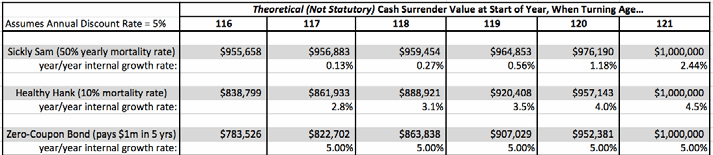
Table 1. Hypothetical Single-Premium (“One-Pay”) Whole Life Policies and Bond Values, With
Death Benefit of $1 Million

I deliberately included the rate of return calculations in Table 1, just so readers would trust me that I’m not hiding anything from them. Yes, those figures are what they are, and this is definitely what’s behind the layperson’s vague worry that “IBC is too expensive for older people.”

Yet hold on. Everything in my analysis last month and this month, assumes friction-less markets where the insurance companies charge actuarially fair premiums, with no premium payment being devoted to overhead, agent commissions, or other miscellaneous items. So, it can’t be that the insurance company is “ripping off” the customer, or that the policyholder is buying a “bad product.” The theoretical market values in Table 1 reflect the fundamentals.

What the doubters are overlooking is that a person who is older and/or in poor health is more likely to get the death benefit sooner rather than later. After all, that’s why the CSVs in Table 1 grow more slowly for Sickly Sam.

Let me show you what I mean. Suppose that Sickly Sam is currently age 120 and is deciding how to allocate his wealth. He can either plunk down $952,381 in a zero-coupon one-year bond that has a face value of $1 million. Or, he can plunk down $976,190 in a whole life policy with a $1 million death benefit.

If Sickly Sam survives another year, then there is a sense in which he would have regretted buying the life insurance policy. He will effectively only earn a 2.44% return on the single premium he paid to take out the policy, whereas he could have earned a 5% return had he invested in the bond instead.

However, we can turn the tables. Suppose Sickly Sam dies right after taking out his whole life policy. Then the executor of his estate would have $1 million that he could invest in bonds that matured into a value of $1,050,000 at the start of year 121. That means Sam’s estate would have earned a return of ($1,050,000 / $976,190) – 1 = 7.6% return (with rounding). So if Sam had instead invested in the bond originally, and then died at the start of Year 120, the executor of his estate would be kicking the now dead Sam, thinking, “If only you would have had the foresight to buy life insurance, I’d have more money to give to your heirs right now.”

Now notice something interesting about those two numbers: If Sickly Sam takes out a whole life policy at age 120, there’s a 50% chance his estate earns a 2.4% return that year, and a 50% chance that his estate earns a 7.6% return. In other words, when we weight the outcomes by their likelihood of happening, then the expected rate of return is…drum-roll please…exactly 5%, which is what Sam would earn if he instead invested in bonds.

This isn’t a coincidence, but instead pops out of the assumptions we built into the analysis underlying Table 1. To keep things apples to apples, we assume the life insurance company invests in the same assets available to others, so everyone is using the same benchmark of a “safe return” (or discount rate). Since the life insurance charges the actuarially fair premiums, given our assumed mortality rates, neither party to a transaction is taking advantage of the other. So, it’s not a surprise that—all things considered, including the possibility of dying—putting money into a life insurance policy has the exact same expected financial rate of return as putting money into a bond fund.

And here ends the extended review of last month’s material. In the remainder of the article, let me extend the above analysis by making the premium payments and mortality rates more realistic.

Keepin’ It Real: Annual Premiums, Earlier Start Date, Actual Mortality Rates

There were many features of last month’s analysis—which we summarized in Table 1 above—that were very unrealistic. So let’s make three changes in this section:

1. We will switch from a one-pay policy to one with a fixed, recurring annual premium.
2. We will have the individual take out the policy at the more relevant age of 50, rather than the extremely old 116.
3. We will now use actual mortality rates, which increase over time, rather than the unrealistic fixed rates of death that we used in Table 1.

With these three changes in mind, consider Table 2. Because we are now showing more years, note that we’ve switched the view from horizontal to vertical. But the logic of the calculations is still the same.

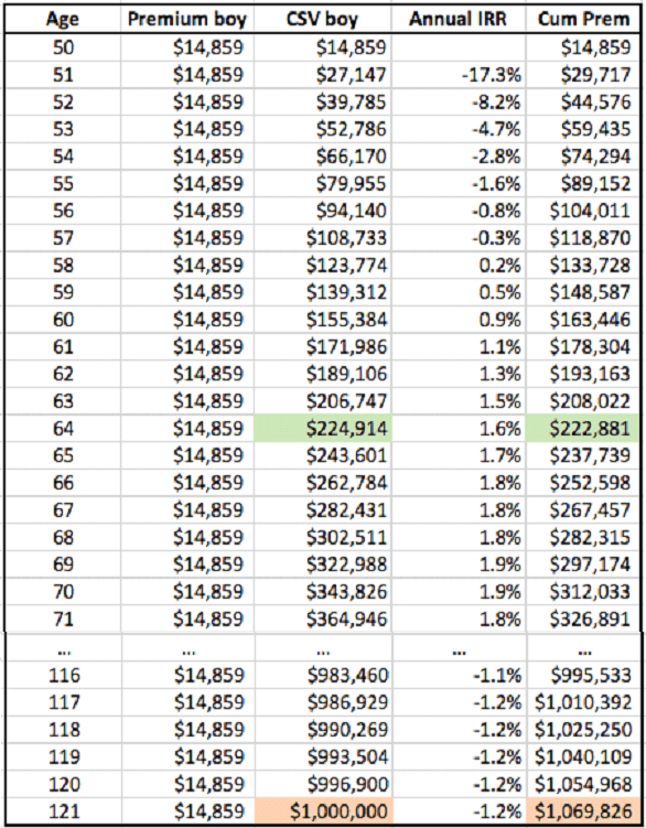
Table 2. Theoretical Cash Surrender Values for Whole Life Policy With Lifetime Annual Premiums
and $1 Million Death Benefit, Using Official Mortality Rates for U.S. Males in 20151
(boy = “beginning of year”)

Although understanding Table 2 is more difficult than Table 1, the principles are the same, and to calculate the Cash Surrender Values, we once again start at the end and work backwards.

There are just two complications: First, the probability of death isn’t a constant number as it was for Sickly Sam or Healthy Hank, but instead are the actual real-world annual mortality rates for a U.S. male (2015) as published by the Social Security Administration. Because of space constraints we haven’t included the numbers in the table, but they start out at 0.32% at age 50, reach 1.07% by age 66, and by age 109 have reached 52.2%— a little worse than Sickly Sam.

The other complication is that at the beginning of each year, a constant premium must be paid to keep the policy in force. This obviously reduces the Cash Surrender Value at any given point, compared to a paid-up policy, because it’s not as valuable to the policyholder to be holding an asset (i.e. a life insurance policy) that requires an influx of future dollars to keep it operational.

We can illustrate what happens by walking through the Year 120 calculation. The annual mortality rate this year is a whopping 94.98%2. However, on the small chance that the insured survives, next year he will have to pay the premium of $14,859 to keep the policy in force, in order to then have access to the face value of $1 million. Therefore, in the event that the individual survives, the net value of the policy to him in Year 120 is ($1,000,000 – $14,859) / 1.05 = $938,230.

Therefore, taking the weighted average of the two possible scenarios (i.e. die or live  in Year 120), the value of the policy at the start of Year 120 is (94.98% x $1 million) + (5.02%  x  $938,230) = $996,900 (with rounding), which is the value shown for Year 120 in Table 2.

As the reader can see in Table 2, the implied “internal rate of return (IRR)” on the Cash Surrender Value starts out negative and then rises. Note that these are annual figures and not cumulative ones. I have marked in green the year when the Cash Surrender Value finally overtakes the cumulative premiums paid in; it’s at that moment when the cumulative return on the policy is positive.

Jumping down to the last few rows of Table 2, we see that the annual (not cumulative) internal rates of return eventually go negative again, which reflects the very high mortality rates for individuals who reach these ages. If a person were to find himself still alive at age 121, he would calculate that since the start of his policy at age 50, he paid in more in premiums than the current value of the policy, i.e. $1 million.

I am showing these results for two reasons. First, I want to remind the reader of what we went through in the previous section, based on Table 1’s values. The calculation of “rate of return” was extremely misleading. From a purely financial viewpoint, in the world described in Table 1, buying life insurance was no better or worse than buying bonds.

There is a similar lesson here, though I will omit the formal calculations. The negative “annual IRR” for the very late years doesn’t show that someone would be foolish to own life insurance at this point. Think of it this way: What are the chances that someone who is still alive at age 115 is still going to be around in six more years? If 10,000 people were alive at age 115, then—according to the SSA’s official mortality rates—only one guy from that group would still be left alive by age 120. And then that guy would only have about a 6% chance of surviving one more year to reach the finish line.

My point here is that it would be extremely unlikely for an individual to actually experience the “Annual IRR” numbers shown at the bottom of Table 2. The vast majority of people would’ve died and gotten their full million-dollar death benefit, much earlier. And when you take this into account, the overall expected financial rate of return on this life insurance policy is…5%, just as before.

The second reason I wanted to show the reader the numbers in Table 2 is that they should reassure doubters that real-world life insurance policy illustrations aren’t merely reflecting agent commissions or other “front-loaded” expenses. The typical whole life policy illustration has a pattern similar to that shown in Table 2, where the internal rate of return on the CSV is very bad early on, but gently rises over time. Since Table 2 does the same thing, even though we have no commissions or other real-world expenses in the calculation, it should reassure us that there are legitimate reasons based on “fundamentals” for the patterns in real-world illustrations.

Front-Loading a Policy Rather Than Relying on Perpetual Premiums

Finally, in this last section I’ll show the theoretical values for a seven-pay whole life policy, in other words a policy where the owner only makes seven premium payments before it is fully funded. As we’ll see, this approach changes the IRR numbers significantly.

This article is already long, so let me just point out the obvious: When a policy is front-loaded, the implied annual (and cumulative, though that’s not shown) internal rate of return is much higher. This doesn’t mean one structure is a “better deal” than another, but I’m just pointing out that the funding approach affects these types of calculations.

These facts are relevant especially for IBC, where the typical policy will combine a contractual base premium for the entire length of the policy, along with a significant amount of Paid-Up Additions early in the policy. To be clear, it’s not the same thing as a contractual 7-pay policy, but real-world IBC policies typically blend both features of what we’ve shown in Tables 2 and 3.

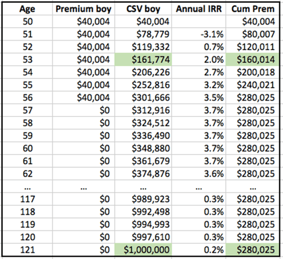
Table 3. Theoretical Cash Surrender Values for Whole Life Policy With Seven Annual Premiums and
$1 Million Death Benefit, Using Official Mortality Rates for U.S. Males in 20153
(boy = “beginning of year”)

Conclusion

The calculations in last month and this month’s articles were theoretical, meaning that I derived them in Excel using simplifying assumptions. The purpose of this exercise was to shed light on how whole life policies actually work, and also to demonstrate that IBC still “works” even for older people or those in poor health.

As we saw, even for those with a high mortality rate, life insurance is still a legitimate “investment” because the higher annual premium is matched by a greater likelihood of getting the death benefit sooner. I also remind the reader that Nelson Nash isn’t telling people to “invest in life insurance,” rather he recommends using life insurance policies as a vehicle to “become your own banker,” i.e. to manage cashflows. Still, I thought it worthwhile to show why the cynics are wrong when they smugly declare that “whole life insurance is a terrible investment.”

Naturally, no reader should make financial decisions based merely on hypothetical tables. The examples I used in these last two articles were intended to teach principles, to help the reader make sense of real-world illustrations. There are many other complicating factors, such as the excellent tax advantages from a properly structured IBC policy, that my simplistic analysis had to ignore.

Anyone who wants to actually apply the theory of IBC to his or her real-life household or business should consult with a graduate from the IBC Practitioner Program that Carlos Lara, Nelson Nash, David Stearns, and I designed. These graduates can be found at: www.InfiniteBanking.org/finder.

References

1. The mortality rates underlying Tables 2 and 3 were taken from the Social Security Administration’s Actuarial Life Table 2015, available at: https://www.ssa.gov/oact/STATS/table4c6.html.
2. Strictly speaking, the SSA mortality figures didn’t include an estimate for age 120, but we took the average mortality rates for ages 119 and 121 to reach the figure cited in the
3. The mortality rates underlying Tables 2 and 3 were taken from the Social Security Administration’s Actuarial Life Table 2015, available at: https://www.ssa.gov/oact/STATS/table4c6.html.